Our original goal was to render a rusty object covered with moss (You can find our original proposal here). While thinking about various approaches to model moss growth, we implemented a point repulsion algorithm (we thought about storing various data in point data structures. Later we decided to render translucent objects using this. Eventually, we ended up implementing weathering and translucent effects. We render both effects in one scene.

Subsurface Scattering (75% Sung Hwan, and 25% Younggon)

First, we implemented a point repulsion algorithm by Greg Turk. The algorithm works as follows :

1. A geometric model (trianglemesh) is read in, and we find three neighbors of each triangle that share an edge. We also compute each triangle's area;

2. Using triangles' areas, we uniformly distribute points across the model surface. The number of uniformly distributed points is determined as "Total_Model_Surface_Area / (PI * mean_free_path)". Here, mean free path is 1/extinction_coefficient of the material.

3. Now, go through each triangle and each point, and rotate neighbor points to the same plane, and compute the overall force on the point.

4. Go through the point list for each triangle again, and then move each point to new locations. If the point moves out of the triangle, find the new triangle that the point belongs to and put it there by projecting the point to the new triangle. The point might be pushed off over more than one triangle.

The following pictures show : an initial distribution over a simple two triangle model, uniformly distributed model, and result of applying the point repulsion algorithm on an entire (closed) model. Different colors were used for points (in a pseudo-random fashion). There are also black pixels in the final image.

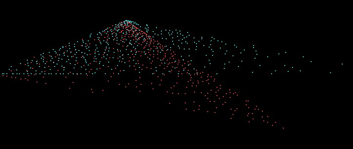
Initial point distribution

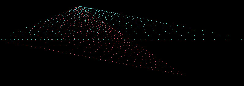
After 20 iterations of point repulsion

After applying to an entire model

Then, we implemented Jensen's hierarchical subsurface scattering technique. Our implementation is done as follows :

1. We use the existing pbrt's photonmap integrator as the base. In the preprocessing step, the photons are stored as usual. Then as we load our model, we load the uniformly distributed points from a file. Then for each point in the model, we interpolate the irradiance at that point using the stored photons.

2. We create an octtree that stores all the irradiance estimates. In each quadrant (besides leaf nodes), we store the overall area (simply sum of all the points' areas), irradiance (sum total flux by adding up multiples of each irradiance estimate and the point's impact area. Then divide the total flux by the total area), and average position (weight each estimate point's position by its irradiance). This estimate of the entire quadrant becomes useful later in speeding things up.

3. When the radiance at a point needs to be estimated (in Li function of the integrator class), we first check whether the object is subsurface or not. If it is, we find the model's corresponding octree, and then compute the subsurface estimate as follows :

- Find whether the point of interest is within the octree's voxel. If it is, pass the request down to its children

- If the point is not inside the voxel, then measure whether the solid angle that subtends to the voxel from the point is within a reasonable limit. If the subtended solid angle is small, then use the quadrant's irradiance, area and point position estimates to compute the irradiance.

- If the subtended angle is too large, break down the voxel into its children and try again (until we reach leaves)

4. After diffusive subsurface scattering estimation, specular reflection is estimated.

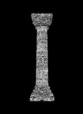
Each leaf in our model can contain upto 8 points. The following pictures show our results. We can play around with scattering/absorption coefficients to get various results, as well as control diffusiveness of surfaces.

Marble column structure

Ketchup dragons with no specular highlights and with specular highlights

Ketchup dragon with area light specular highlights

A flow simulator is built to simulate the flow pattern. Water is modeled as a particle which moves on a surface. Because the canon model we got had several meshes, the simulator had to work with arbitrary number of meshes. The hard problem was to find an adjacent triangle as a particle move on. Instead of building a new scheme or data structure, ray tracing capability of pbrt was used.

In one iteration, a particle moves a small predefined distance of 2.5 mm. The simulator shoots a ray to check if there is a contact. If the ray meets other triangle, the particle will flow following the edge between two surfaces. It also shoot a ray to downward to check if the particle is still on the same triangle. If not, the particle will free fall to ground or stick to other triangle.

The simulation for a particle ends when it falls on a ground or the number of iteration is over five hundreds. The particle can be stuck at concave shape.

The cost of having 2 ray tracings per iteration was tolerable. It took less than 3 hours to generate a half million traces. Following figure shows the simulator integrated in pbrt and glut (flow.cpp)

Several random elements are introduced to generate more natural patterns. Rain direction (blue line above) is changed by random amount to model wind. Also free fall direction is modulated to generate a wide spread stain pattern. Lastly, gravity direction is slightly modulated to make the flow pattern more random and natural. It also make the particle flow on a surface parallel to ground, which happens a lot in artificial model.

The profile of the flow is recorded on the subdivided triangle mesh. Each triangle records how many times particles have passed on itself. This profile is post-processed to generate rendering file (ground.cpp, surface.cpp). Simplifying assumptions are made - the more particle passed on the spot, the more likely it has stain.

Two options were explored to render the stain - using texture and micro geometry. The density of stain is converted to exr texture file and used to modulate the texture color. Due to the difficulty of generating uv coordinate, this scheme is experimented only on ground. The resulting picture was flat compared to the second option. In second option, a large number of spheres are used to draw stain. The result was more convincing. The drawback is large pbrt file size. The rendering time was affected less than factor of two.

Here is a mapping used to calculate radius of sphere given the contact counting. The triangle which is contacted more often will have larger sphere on it.

To give more variety on the color of stain, two different colors were used - normal color (0.25, 0.1, 0.1) and darker color (0.15, 0.1, 0.1).  Each sphere randomly choose darker color. The probability increases as count increases, to give a darker color on dense stain region.

Here is a final image. Marble texture built in pbrt and bump mappoing were used to render ground.

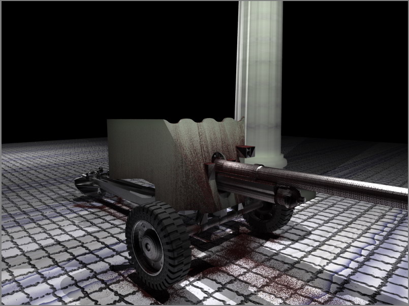Although it is not very obvious, the shield of the gun is also done using subsurface scattering in this picture.

Our source code can be found here.