 |
|
|
|
For each of the light fields, we provide:
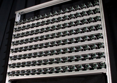
Camera-id X YFor light fields acquired using the computer-controlled gantry, we provide the same information. The only difference is that the camera positions are obtained from the gantry instead of parallax measurements. The camera positions are in millimeters and our gantry is sub-millimeter accurate.
Light fields acquired with the lego gantry are treated similarly to the camera array. The blue/yellow corners visible in the original images define the reference plane, and the red/green corners determine parallax. This computed parallax, which is related to the center of projection of the camera by an unknown scale and translation, is included as part of the file name of each rectified image, in the order (Y, X), so that lexicographic sorting of the files produces a row major ordering of camera images. Computed homographies are not included, but are easy to compute from the original images using basic computer vision techniques (corner detection and some linear algebra to compute the 3x3 homography).
Our calibration error is less than 0.5 pixels. This error is primarily due to uncertainity in corner detection. A quantitative analysis of the error may be found in [2], Appendix A.
Calibration for the light field microscope images is a fairly different process, as the microlens array records the 4D transpose of what a gantry or camera array records. The main step is rotating and scaling the image of the microlens array so that it becomes axis-aligned, with each microlens having an integral width and height. However, optical aberrations come into play both within each lenslet and across the lenslet array. For more details, see the Stanford Light Field Microscopy project web page.
© 2008 Stanford Graphics Laboratory
Created by Vaibhav Vaish. Updated by Andrew Adams.
Last update:
June 6, 2008 05:41:59 PM